
This post walks through implementing Mario Klingemann’s Stack Blur algorithm, a CPU image blurring algorithm. It’s the post I wish I had while building my vectorized C++ blur for the JUCE framework.
Go straight to the implementation section, or check out the Benchmarks.
Why CPU blurring and what is Stack Blur?
There are still times and places in 2023 where access to the GPU isn’t available or is convoluted. In these cases, Stack Blur is used (quite widely) for efficiently blurring images on the CPU.
In my case, I’m building cross-platform audio plugins with the JUCE framework. OpenGL is available, but deprecated and crusty on macOS. And it’s a can of worms I’d prefer not to open when all I want are some drop shadows and inner shadows (so I don’t have to use image strips like it’s the 1990s).
This is an example of a slider control in my synth:

3 inner, 2 drop shadows for the level indicator.
3 drop shadows for the slider “thumb.”
It’s vector-only and “brought to life” via 10 drop shadows and inner shadows that provide depth and lighting. There are up to 10 of these on a page, animating at 60 frames per second, along with lots of other UI. So they need to be fast.
A true gaussian image blur is quite expensive: CPU time scales up with both image size and radii. That makes the Stack Blur algorithm a perfect fit for places where GPU access is limited or unavailable.
Gaussian is a fancy synonym for a “normal distribution”. That’s statistics jargon for “bell curve-like”. In our context, to get a nice blur, we want each pixel to be affected by all the closest pixels surrounding it. The “influence” from these neighboring pixels tapers off like a bell curve.
Before describing what the algorithm does, I’ll walk through some fundamental concepts.
Single Channel Stack Blur
We’ll start by handling an image format that’s a single color, or single channel. Single channel images are what’s used under the hood to make drop shadows. Each pixel is just one value: brightness (later composited with a specified color).
Our brightness pixel values go from 0 to 255. So each pixel is stored as 8 bits. (In C++ this would be the uint8_t or unsigned char).
Here’s what our image might look like with some arbitrary values:
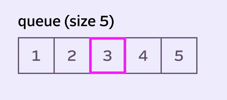
The Stack Blur Queue concept
In the world of image convolution (for example, gaussian blurring) there’s a 2D matrix that slides over the image. It uses fancy dot product magic [insert some hand waving] to calculate the result of the center pixel.
GPUs are great at parallelizing this kind of convolution. CPUs not so much.
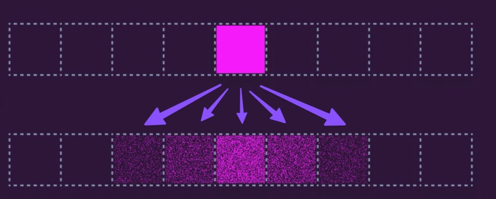
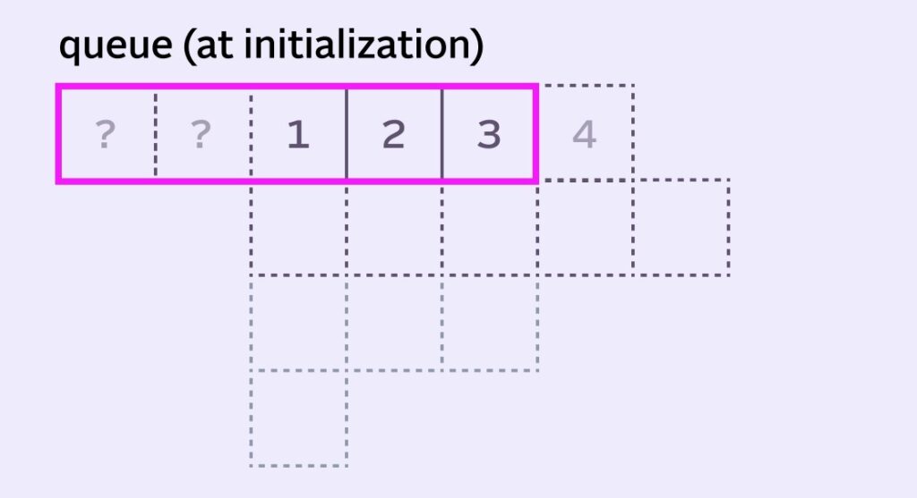
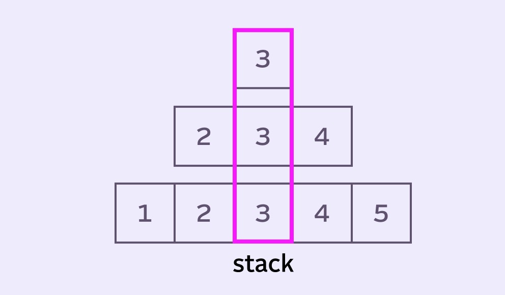
Stack Blur is different. It operates one row (or column) at a time (simulating 1D convolution) using weighted sums. Instead of living the fancy matrix life, we’re chilling with a humble array of values that Mario called the queue (in image convolution it’s usually referred to as a kernel).
We’ll use the queue/kernel surrounding the pixel to perform some magic 🪄 to calculate the blurred value for the center pixel. In the illustration above, we’re calculating the blur value the center pixel (255) using the 5 pixels in the queue. We’ll get into the exactly how a bit later.
Because we always need a pixel at the center of the queue (the one we are blurring), our queue size is always odd-numbered. That means we can think in terms of a blurred pixel having a radius.
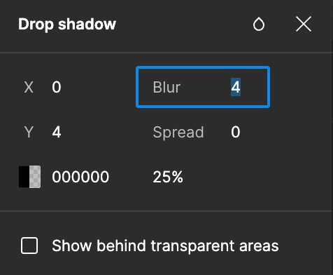
In our example, the radius is 2: we have 2 pixels on either side of the center pixel. Specifying radius is also how people normally specify blur when designing for the web and in design programs such as Figma:
Our total queue size is double the radius plus our center pixel. queueSize = radius*2 + 1 or 5.
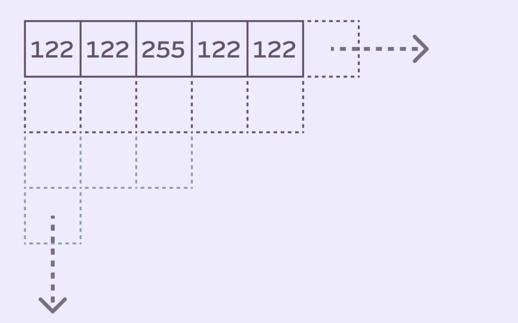
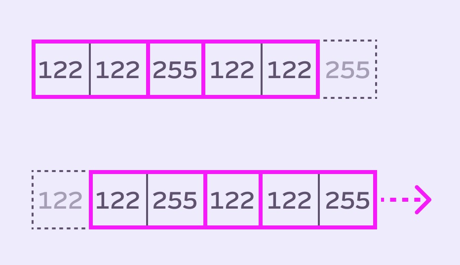
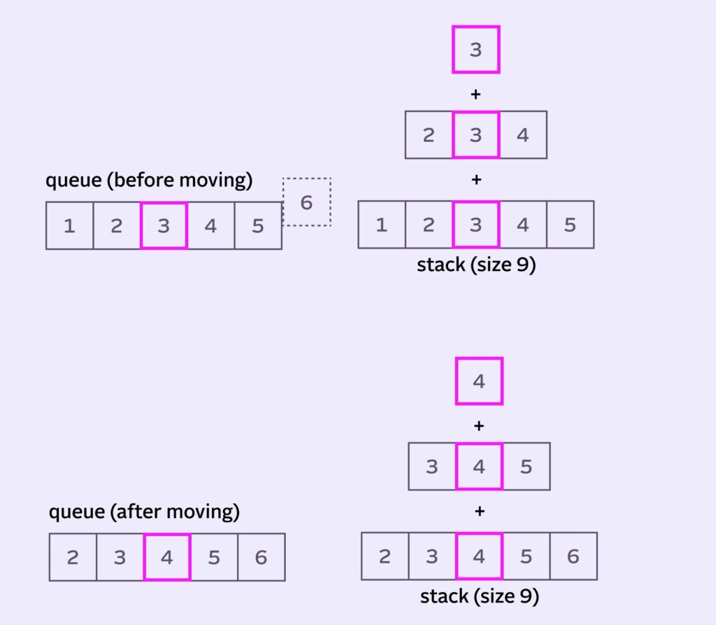
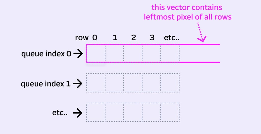
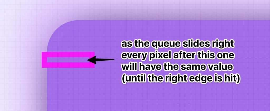
When we want to process the next pixel, we slide our queue across the row of pixel values in the image. The queue gains the pixel from the right hand side and loses the leftmost pixel:
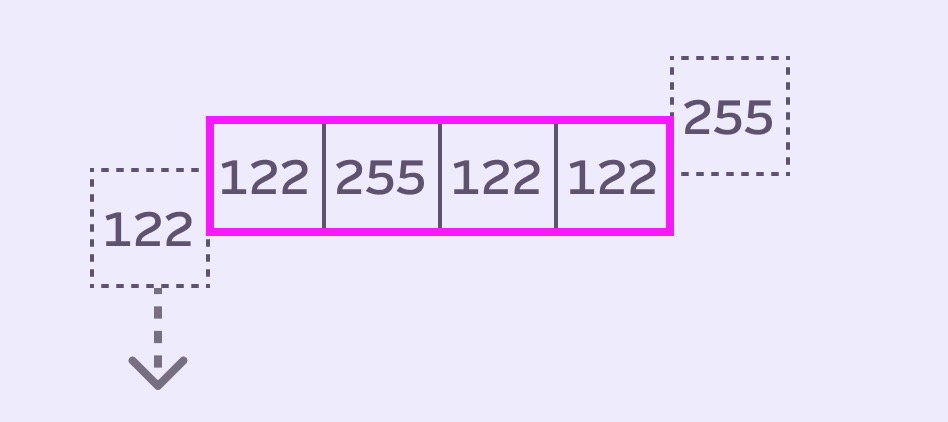
You can also imagine this process from the queue’s point of view, as Mario illustrates:
Stack Blur Queue Implementation
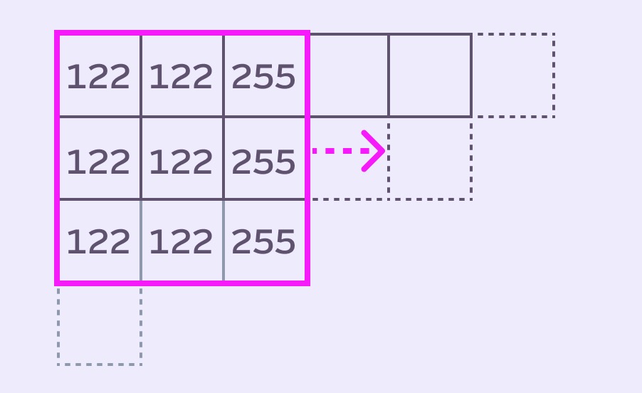
Let’s keep looking at things from the queue’s point of view.
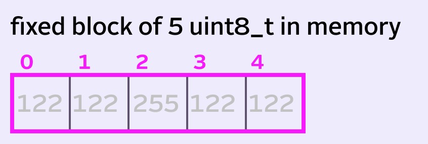
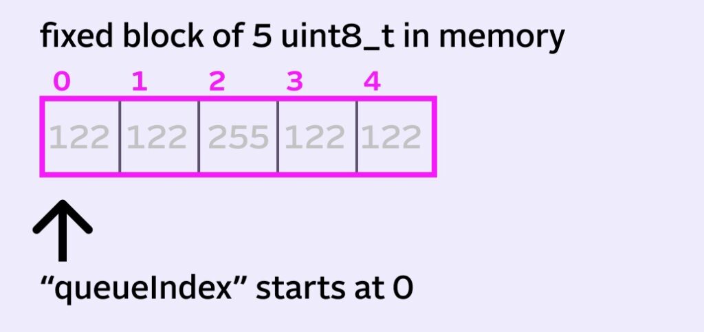
With a radius of 2, we have a queue size of 5. That means technically we only need 5 pieces of memory for our queue. We’ll give each piece of memory a 0-based index, just to be clear going forward.
When a new value comes onto the queue, the leftmost value is removed. The other values then all move left one spot to make room for the incoming value.
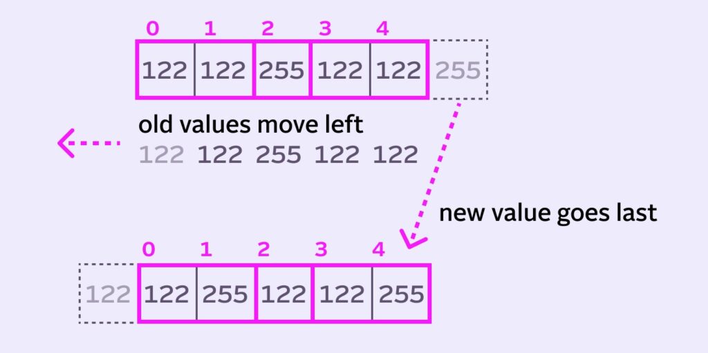
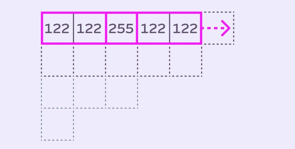
255 center pixel moves from index 2 to index 1.This is trivial to implement with something like std::deque in C++:
queue.pop_front(); // get rid of leftmost pixel
queue.push_back (incomingValue); // add new pixel
However, it’s also inefficient. Each time the queue slides, every value in the queue has to change position in memory. This is a lot of work to do per-pixel. It scales up poorly for larger radii.
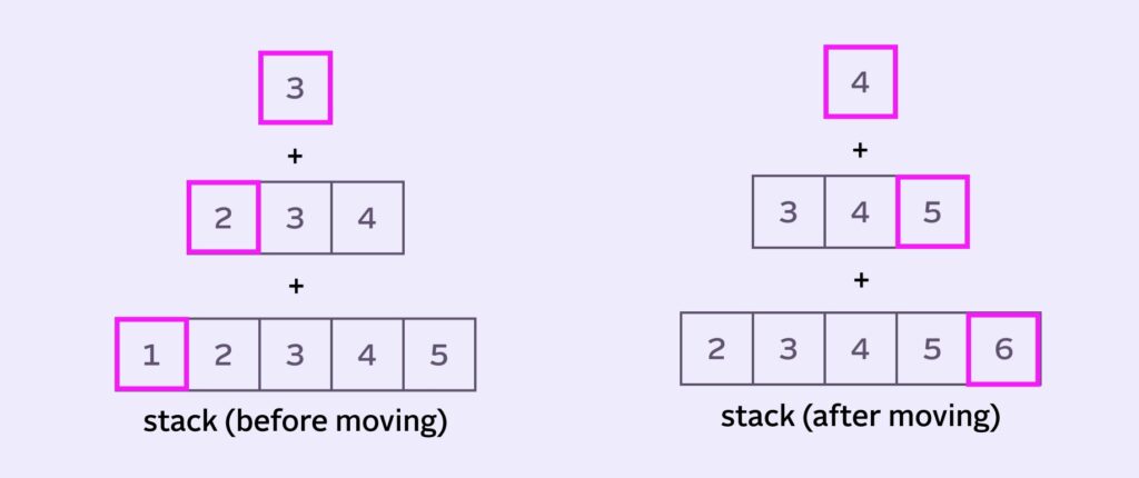
Circular Buffer Implementation
The efficient thing to do is implement a circular buffer, sometimes called a ring buffer. It’s often called a FIFO (First In, First Out) by audio programmers.
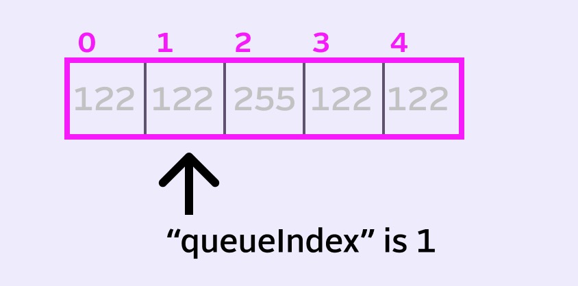
The trick is to abstract our queue from its physical memory by using another variable, such as queueIndex. This index will specify where our new fancy virtual queue starts.
When we move to the next pixel, instead all the values shifting left, we’ll just increment the index and move it one spot over to the right.
Conveniently, the incoming pixel can replace the pixel at old queue index, which is now the end of our virtual queue.
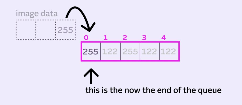
Now, when we want to read our full queue, we can now start at queueIndex and read the next 5 pixels, wrapping back to the beginning when we hit the end of the memory block. This wrapping back to the 0 index is why it’s called a circular/ring buffer.
Stacking the Bricks
Let’s get into the magic. ✨
We want to emulate a smooth gaussian blur in which a pixel is more affected by its closest neighbors.
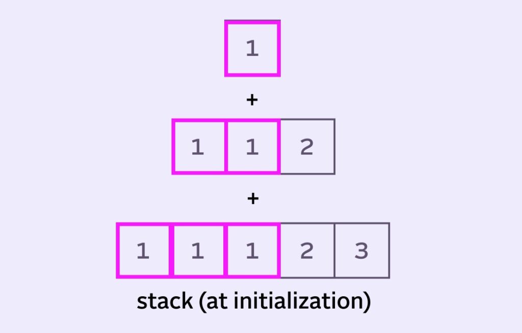
Mario’s accomplishes this with a concept he calls a stack. He notes the stack isn’t a real structure (in terms of memory or even implementation). The goal is just to give a heavier weight to the center pixel in the queue. And taper the influence off as we move away from the center.
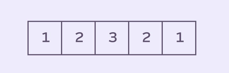
To illustrate, let’s assign some unique pixel values to our simple queue:
To calculate the blur for the center pixel, we could just take the average of all pixels in the queue: (1+2+3+4+5) / 5 (which just happens to equal 3, lulz). This is exactly how a Box Blur is implemented. Unfortunately Box Blur is both inefficient and doesn’t look great.
So how can we give additional emphasis to the pixels around the center to make it more smooth and bell-curve-y? Well, one idea is to make a copy of the queue, reduce the diameter and include this new layer in our calculations. And keep stacking layers until we’re left with a single center pixel layer:
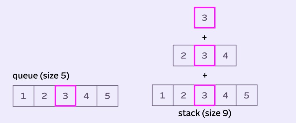
Welcome to Stack Blur. It “stacks” smaller and smaller virtual queues on top of each other, which gives heavier weight to pixels closest to the center of the queue.
Ironically, in this example (1+2+2+3+3+3+4+4+5) / 9 actually ends up equalling 3 again! All that hard work for nothing :). Don’t rage quit and close the browser yet, here’s a better example:
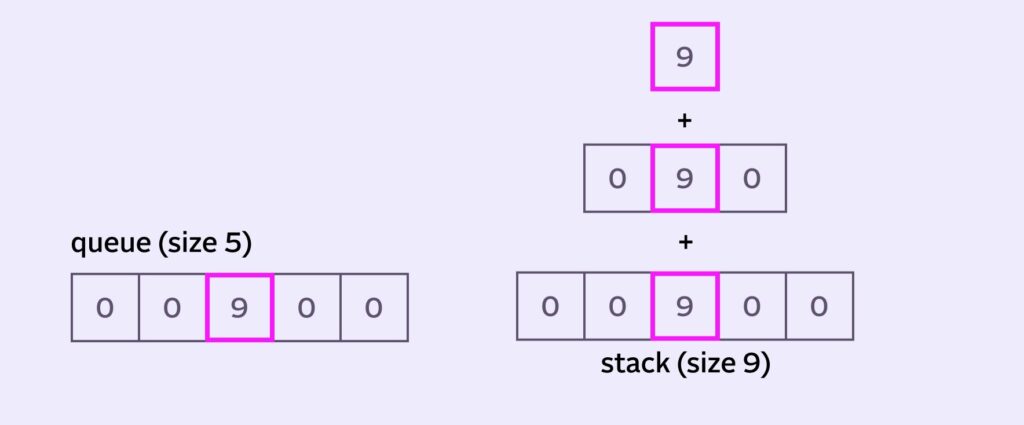
The average of the queue is (0+0+9+0+0)/5 = 1.8. But the average of the stack is (0+0+0+9+9+9+0+0+0)/9 = 3. So the result is skewed towards our higher center pixel value.
Stack Blur Implementation
Remember: the stack isn’t real. Keeping all those extra pixel values around would be too much bookkeeping and number crunching. Instead, we’ll implement a moving average, a sum that we will call stackSum.
How do we alter the stackSum when the queue moves? When we look closely, the stack seems to gain and lose a bunch of different values.
It’s easiest to think the state both before and after the queue moves.
It seems like we can find our answer on the edges of the stack
1+2+3 and 4+5+6 at the “edges” of the stack.sumOut is everything we’ll remove from the stack each iteration. In our, example it is 1+2+3.
sumIn is what we need to add to the stack. In our example it’s 4+5+6.
But wait! The stack is all in our head, maaaaan. So how exactly do we get the actual values? Let’s take a closer look at our queue:
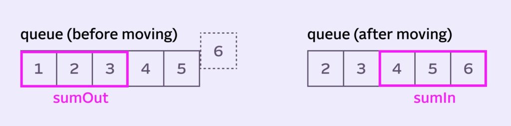
1+2+3 and 4+5+6Oh wait, it’s right there in the queue. But again, we can’t constantly be summing individual pixels. So sumIn and sumOut are also running sums. That way, all we have to do on each move is:
- add and subtract a number from
sumInandsumOut - modify
stackSumby addingsumInand removingsumOut
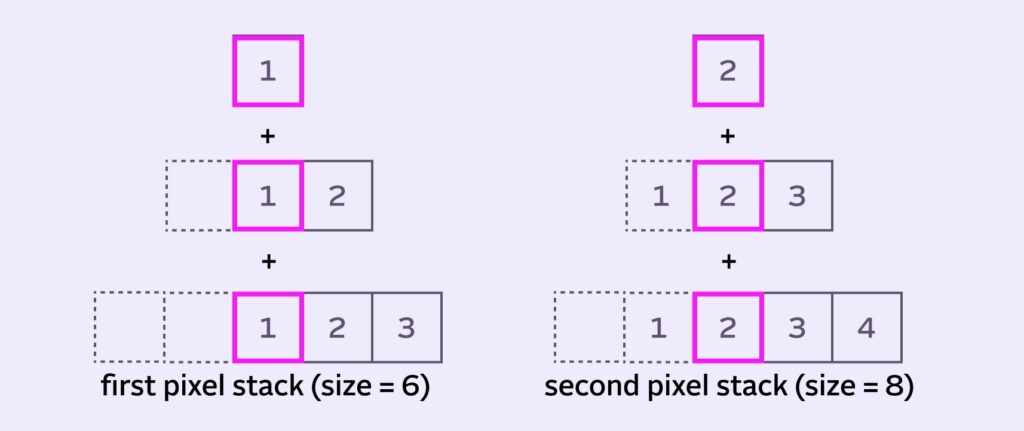
Implementing each stack move
There are different ways of implementing this, but if we’re optimizing for tracking and storing the fewest number of pixels, here’s a good workflow:
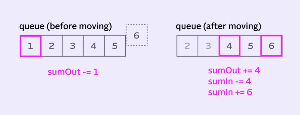
- Calculate the blur for the current center pixel with
stackSum/stackSize - Remove
sumOutfromstackSum - Before moving,
sumOutloses the leftmost pixel (or the pixel atqueueIndex):1 - We move the queue, adding the incoming
6and removing the old and tired1 sumIngains the incoming new pixel6- After moving,
sumOutgains the incoming4, which is the the new center pixel (atqueueIndex + radius) sumInloses that same new center pixel4
You can see a code implementation here. That certainly feels like more work than “adding and subtracting a value from the queue”. But it’s also surprisingly few instructions for a lot of heavy lifting. And most importantly, the number of instructions per pixel stays constant, no matter how large the radius gets.
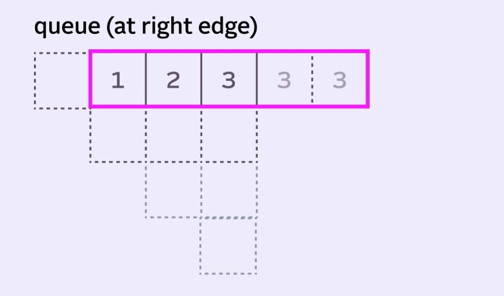
Literal Edge Cases
What to do when the pixel we want to calculate is at the edge of an image? This is pretty important — the edge is where we’re starting from! We’ll have to invent some numbers for the leftmost pixel and for sumIn and sumOut, won’t we?
Most implementations pre-populate the left side of the queue with the leftmost pixel value. So our example imaginary stack would initialize like this:
sumOut starts with the sum of the 6 highlighted pixels (6 here).
sumIn can be initialized with the remaining pixels from the stack (value of 7).
We do the exact same thing when approaching the right edge, reusing that last pixel to fill the queue as needed.
This works fine, but does create a bias towards those edge pixels. The “influence” of the edge pixels creates what’s called edge bleed.
For a more accurate blur, some implementations will vary the denominator (aka, vary the stack size) for the edge pixels. Varying the denominator with our radius of 5, the stacks for the first two pixels would look like this:
Horizontal and Vertical Stack Blur passes
Like the Box Blur algorithm, we want to approximate a 2D gaussian kernel blur. We do that by running 2 passes over the image: one horizontal and one vertical. The vertical pass operates on the result of the horizontal pass, compounding the blur.
Job van der Zwan has a post on Stack Blur with a great interactive (!) visualization of how sliding the stack in two passes ends up simulating a gaussian-esque 2D kernel.
Multi-channeI images
Luckily, dealing with multi-channel images is conceptually identical to single channel images.
At the low level, most images on consumer operating systems are stored in a native interleaved pixel format. That just means: each of the 8-bit values for Red, Green, Blue, Alpha (transparency) that comprise “one pixel” are stored together in memory (into a 32-bit space).
There are important implementation details around scary sounding things like “little endian” storage of pixel values and “premultiplied alpha”. But basically, the pixels are packed together in a BGRA order on Windows and MacOS.
Why does Stack Blur work, though?
If we look at our stack and pay attention to the columns, we might start to understand how exactly the stack gives weight to the pixel values. In our example, the center pixel shows up 3 times, the pixel on either side 2 times and the edge pixels once.
3 is being added radius + 1 times.What if we just try to do something with these weights? Here are the weights for the stack above:
stackSizeWe can normalize the weights by dividing by the stackSize. That would let us apply them to directly to pixel values.
Interesting! Notice that the full value (9/9) of a pixel is distributed across all 5 places where the pixel is relevant! We can finally sorta understand how Stack Blur blurs.
This kernel of abstract pixel weights seems… interesting. Can we just use it somehow? Yes, but we’d have to multiply the kernel against the queue value by value. And a queueSize number of multiplications per pixel doesn’t sound too ideal…
Plus, isn’t this starting to smell a bit like an expensive convolution kernel we’re trying to avoid? 🙈
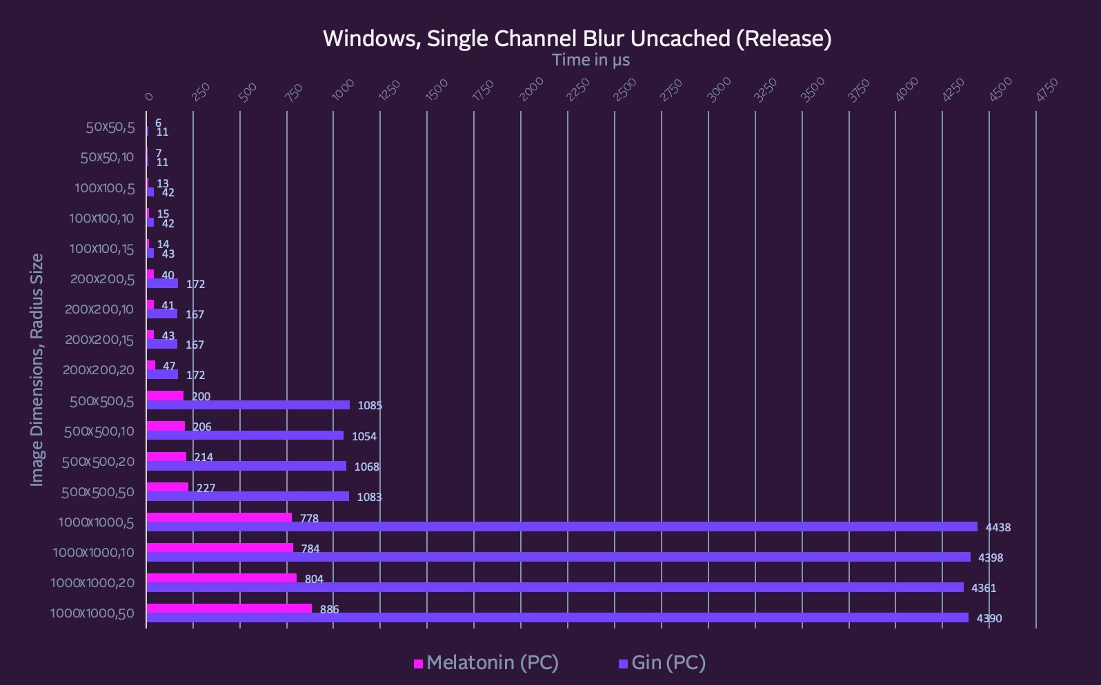
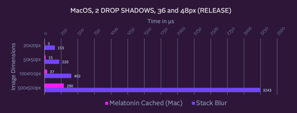
The part where I test, implement and benchmark 15 Stack Blur implementations

I wanted to make sure I was getting the fastest performance possible. I don’t want to worry about hundreds of drop shadows suddenly making my synth perform worse (especially on Windows).
As I keep saying, Stack Blur’s primary optimization is ensuring there are the same number of operation per pixel when the radii scales. But my real life usage (using drop and inner shadows to build UI), radii are usually in the 4-36px range. So perhaps the algorithm is over-optimized for radii size?
Also, the original Stack Blur algorithm was made for an environment without access to SIMD or Intel/Apple vector libraries (Javascript, in 2004). Vector processing and SIMD options have come a long way since then.
These days there are some fancy and fast libraries for convolution in C++, such as Apple’s Accelerate and Intel’s IPP. Surely these vendor libraries have some tricks up their own sleeve? Sure, maybe a full blown vector accelerated gaussian blur will be too expensive (spoiler: it is), but what if we do two passes of vector x matrix convolution?
Well, fast forward a couple weeks and 20+ implementations later (and counting) and yes: both Apple and Intel’s vector libraries are quite a bit faster for Single Channel Images. Full benchmarks here.
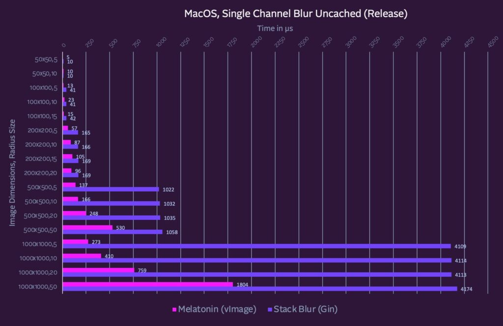
The long story: For the most image and radii sizes, vendor libraries (employing SIMD, etc under the hood) outperform Stack Blur, especially as the image dimensions scale up.
Starting with macOS 11.0, Apple has vImageSepConvolve for separated passes, which basically beats stack blur in a couple lines of code.
Intel’s offerings were less exciting. I have a graveyard of failed Intel attempts to use things like ippiFilterSeparable, their separable kernel offering. Pretty sure it’s doing 2D convolution under the hood, because performance is killed by larger radii.
I did write a fast single channel vector IPP Stack Blur which performs decently:
It “rotates” the queue so that you have n vectors where n is your queue size and they are filled with the entire column (for the horizontal pass) or row (for the vertical pass).
However, it turns out that the C++ Stack Blur implementation I’ve been using is already very optimized.
There are also cases where Stack Blur outperforms everything I tried (I still haven’t found an algorithm faster than it for ARGB images on Windows).
So, can I use hundreds of CPU made drop shadows to build my UI? Yes. The real trick is to render the shadow once and cache it for future repaints. That brings shadow repainting time down to almost raw image compositing levels. Getting fast initial paints is still worth it though! Especially for anything animating. At least what I tell myself to sleep well at night 🙂
Other Stack Blur optimizations
One obvious optimization for drop shadows in particular is that the larger the image dimensions, the less of the image is actually relevant to the end result. In other words, content is drawn on top of the drop shadow, so we don’t care about the middle. Only the edges need to be blurred. Someone in the comments can probably provide a formula for this.

A Stack Blur optimization for this is what I call the “Martin optimization,” named after my father-in-law. I sat down with him and my wife (both extremely logical thinkers who play code optimizing video games!) and asked them how they’d optimize the algorithm. One of his insights was that if the values in the queue were all the same and the next incoming pixel was that same value, it’s a no-op: the algorithm can be skipped for the incoming pixel.
When rendering drop shadows to a graphics context, the inside rectangle of the single color filled path can also be clipped out, saving compositing time.
Further exploring the convolutional roots
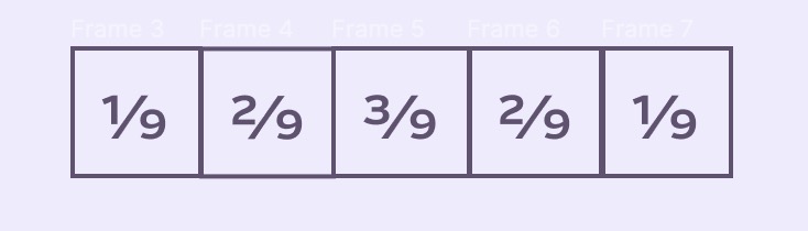
Another interesting tangent my wife and I went on:
If we focus on the relative weight of a pixel as it moves through the queue, we can see the first time the pixel enters the queue, its weight is 1/9. When it moves, the weight doubles to 2/9, then it’s multiplied by 3/2 to for a weight of 3/9. As it moves into the right side of the kernel, it shrinks, first by 2/3 and then by 1/2.
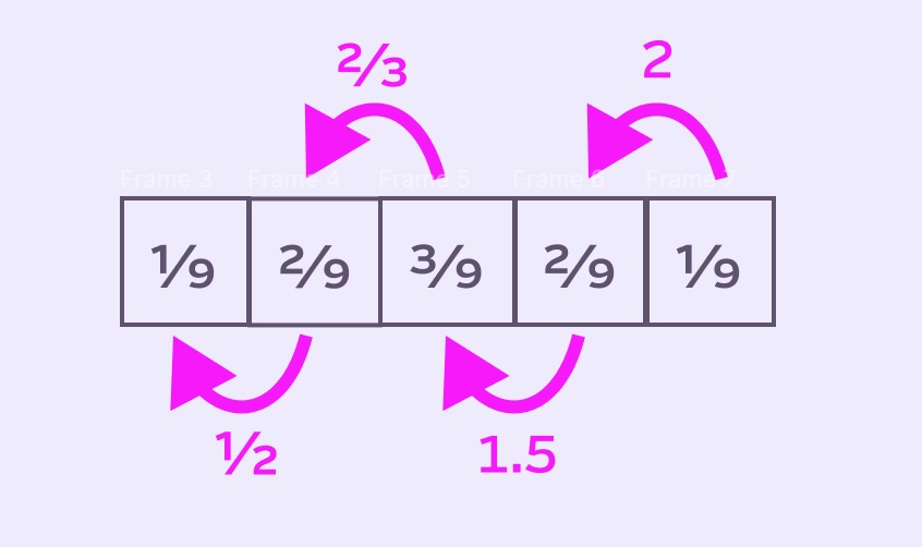
So we could look at the multipliers that describe a single pixel’s “journey” through the queue:
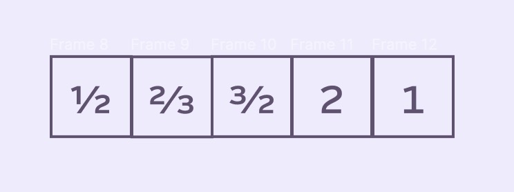
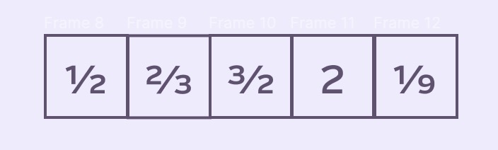
We can then normalize for any queue size by scaling the rightmost pixel upon entry to the queue. For our stackSize of 9, let’s have it scale the incoming pixel by 1/9:
This looks promising! But what can we do with it? Using it against the queue would save us from 4 add/subtracts per queue move and having to read and write to sumIn and sumOut — but we gain 5 multiplies (and more as the radius scales up).
Well, the answer is I have no idea how this could be useful. Please let me know in the comments if you have ideas 🙂
Stack Blur Implementations and Resources
- My C++ implementations for the JUCE framework
- Mario’s original implementation notes
- Blog post about solving the edge problem with varying the denominator
- Job van der Zwan’s modern JS implementation with great visualizations
- LoganDark’s Rust implementation which solves edge bleed

Leave a Reply